GRACE TECHNICAL REPORTS
Marker-directed Optimization of UnCAL
Graph Transformations
Soichiro Hidaka
Zhenjiang Hu
Kazuhiro Inaba
Hiroyuki Kato
Kazutaka Matsuda
Keisuke Nakano
Isao Sasano
GRACE-TR 2011–02
June 2011
CENTER FOR GLOBAL RESEARCH IN
ADVANCED SOFTWARE SCIENCE AND ENGINEERING
NATIONAL INSTITUTE OF INFORMATICS
2-1-2 HITOTSUBASHI, CHIYODA-KU, TOKYO, JAPAN
Marker-directed Optimization of UnCAL Graph
Transformations
⋆Soichiro Hidaka1, Zhenjiang Hu1, Kazuhiro Inaba1, Hiroyuki Kato1, Kazutaka Matsuda2, Keisuke Nakano3, and Isao Sasano4
1
National Institute of Informatics, Japan,
{hidaka, hu, kinaba, kato}@nii.ac.jp
2
The University of Electro-Communications, Japan, [email protected]
3 Tohoku University, Japan,
4
Shibaura Institute of Technology, Japan, [email protected]
Abstract. Buneman et al. proposed a graph algebra called UnCAL
(Un-structured CALculus) for compositonal graph transformations based on structural recursion, and we have recently applied to model transfor-mations. The compositional nature of the algebra greatly enhances the modularity of transformations. However, intermediate results generated between composed transformations cause overhead. Buneman et al. pro-posed fusion rules that eliminate the intermediate results, but auxiliary rewriting rules that enable the actual application of the fusion rules are not apparent so far. UnCAL graph model includes the concept of mark-ers, which correspond to recursive function call in the structural recur-sion. We have found that there are many optimization opportunities at rewriting level based on static analysis, especially focusing on markers. The analysis can safely eliminate redundant function calls. Performance evaluation shows its practical effectiveness for non-trivial examples in model transformations.
Keywords:program transformations, graph transformations, UnCAL
1
Introduction
Graph transformation has been an active research topic [8] and plays an impor-tant role in model-driven engineering [5, 10]; models such as UML diagrams are represented as graphs, and model transformation is essentially graph transfor-mation. We have recently proposed a bidirectional graph transformation frame-work [6] based on providing bidirectional semantics to an existing graph transfor-mation language UnCAL [4], and applied it to bidirectional model transforma-tion by translating from existing model transformatransforma-tion language to UnCAL [9]. Our success in providing well-behaved bidirectional transformation framework
⋆This is a full version of the paper to apper in Proc. of The 21st International
was due to structural recursion in UnCAL, which is a powerful mechanism of visiting and transforming graphs. Transformation based on structural recursion is inherently compositional, thus facilitates modular model transformation pro-gramming.
However, compositional programming may lead to many unnecessary inter-mediate results, which would make a graph transformation program terribly in-efficient. As actively studied in programming language community, optimization like fusion transformation [11] is desired to make it practically useful. Despite a lot of work being devoted to fusion transformation of programs manipulating lists and trees, little work has been done on fusion on programs manipulating graphs. Although the original UnCAL has provided some fusion rules and rewrit-ing rules to optimize graph transformations [4], we believe that further work and enhancement on fusion and rewriting are required.
The key idea presented in this paper is to analyze input/output markers, which are sort of labels on specific set of nodes in the UnCAL graph model and are used to compose graphs by connecting nodes with matching input and output markers. By statically analyzing connectivity of UnCAL by our marker analysis, we can simplify existing fusion rule. Consider, for instance, the following existing generic fusion rule of the structural recursion in UnCAL:
rec(λ($l2,$t2).e2)(rec(λ($l1,$t1).e1)(e0))
=rec(λ($l1,$t1).rec(λ($l2,$t2).e2)(e1@rec(λ($l1,$t1).e1)($t1)))(e0)
whererec(λ($l,$t).e) denotes a structural recursive function which is an impor-tant computation pattern and will be explained later. The graph constructor@ connects two graphs by matching markers on nodes, and in this case, result of transformatione1is combined to another structural recursionrec(λ($l1,$t1).e1). If we know by static analysis that e1 creates no output markers, or equiva-lently,rec(λ($l1,$t1).e1) makes no recursive function call, then we can eliminate @rec(λ($l1,$t1).e1)($t1) and further simplify the fusion rule. Our preliminary performance analysis reports relatively good evidence of usefulness of this opti-mization.
The main technical contributions of this paper are two folds: a sound and refined static inference of markers and a set of powerful rewriting rules for op-timization using inferred markers. All have been implemented and tested with graph transformations widely recognized in software engineering research. The source code of the implementation can be downloaded via our project web site atwww.biglab.org.
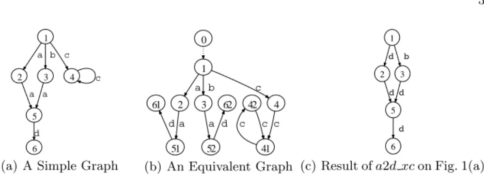
1 2 a 3 b 4 c 5 a a c 6 d
(a) A Simple Graph
0 1 2 a 3 b 4 c 51 a 61 52 a 62 41 c 42 c d d c
(b) An Equivalent Graph (c) Result ofa2d xcon Fig. 1(a)
Fig. 1.Graph Equivalence Based on Bisimulation
2
UnCAL Graph Algebra and Prior Optimizations
In this section, we review the UnCAL graph algebra [3, 4], in which our graph transformation is specified.
2.1 Graph Data Model
We deal with rooted, directed, and edge-labeled graphs with no order on outgoing edges. They are edge-labeled in the sense that all information is stored on labels of edges while nodes have no labels. UnCAL graph data model has two prominent features, markers and ε-edges. Nodes may be marked with input and output markers, which are used as an interface to connect them to other graphs. An ε-edge represents a shortcut of two nodes, working like the ε-transition in an automaton. We useLabel to denote the set of labels andMto denote the set of markers.
Formally, a graph G, sometimes denoted by G(V,E,I,O), is a quadruple
(V, E, I, O), where V is a set of nodes,E ⊆V ×(Label∪ {ε})×V is a set of
edges, I ⊆ M ×V is a set of pairs of an input marker and the corresponding node, andO⊆V × Mis a set of pairs of nodes and associated output markers. For each marker&x ∈ M, there is at most one nodev such that (&x, v)∈I. The node v is called aninput nodewith marker &x and is denoted by I(&x). Unlike input markers, more than one node can be marked with an identical output marker. They are calledoutput nodes. Intuitively, input nodes are root nodes of the graph (we allow a graph to have multiple root nodes, and for singly rooted graphs, we often use default marker & to indicate the root), while an output node can be seen as a “context-hole” of graphs where an input node with the same marker will be plugged later. We write inMarker(G) to denote the set of input markers andoutMarker(G) to denote the set of output markers in a graph
G.
V = {1,2,3,4,5,6}, E = {(1,a,2),(1,b,3),(1,c,4),(2,a,5),(3,a,5),(4,c,4), (5,d,6)}, I = {(&,1)}, and O = {}. DBXY denotes graphs with sets of input
markersX and output markersY. DB{Y&} is abbreviated toDBY.
2.2 Notion of Graph Equivalence
Two graphs are value equivalent if they are bisimilar. Please refer to [4] for the complete definition. Informally, graphG1 is bisimilar to graphG2 if every node x1 in G1 has at least a bisimilar counterpart x2 in G2 and vice versa, and if there is an edge fromx1 to y1 in G1, then there is a corresponding edge from x2 to y2 in G2 that is a bisimilar counterpart ofy1, and vice versa. Therefore, unfolding a cycle or duplicating shared nodes does not really change a graph. This notion of bisimulation is extended to cope with ε-edges. For instance, the graph in Fig. 1(b) is value equivalent to the graph in Fig. 1(a); the new graph has an additional ε-edge (denoted by the dotted line), duplicates the graph rooted at node 5, and unfolds and splits the cycle at node 4. Unreachable parts are also disregarded, i.e., two bisimilar graphs are still bisimilar if one adds subgraphs unreachable from input nodes.
This value equivalence provides optimization opportunities because we can rewrite transformation so that transformation before and after rewriting produce results that are bisimilar to each other [4]. For example, optimiser can freely cut off expressions that is statically determined to produce unreachable parts.
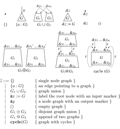
2.3 Graph Constructors
{} {a : G}
G a
G1 ∪G2
G1 G2 G
&z := G &z
&z ()
&x1 ... &xm
&y1 ... &yn
&x1’ ... &xm’
&y1 ... &yn
G1 G2
G1G2 G1@G2
&x1 ... &xm
&y1 ... &yn
G1
&z1 ... &zp
&y1 ... &yn
G2
ε ε
cycle(G)
&x1 ... &xm
&x1 ... &xm
&x1 ... &xm
ε G ε
&z
ε ε
&x1 ... &xm
G::={} {single node graph}
| {a:G} {an edge pointing to a graph} | G1∪G2 {graph union}
| &x:=G {label the root node with an input marker} | &y {a node graph with an output marker} | () {empty graph}
| G1⊕G2 {disjoint graph union} | G1@G2 {append of two graphs}
| cycle(G) {graph with cycles}
Fig. 2.Graph Constructors
Example 1. The graph equivalent to that in Fig. 1(a) can be constructed as follows (though not uniquely).
&z@cycle((&z :={a:{a:&z1}} ∪ {b:{a:&z1}} ∪ {c:&z2}) ⊕(&z1 :={d:{}})
⊕(&z2 :={c:&z2})) ⊓⊔
For simplicity, we often write{a1 : G1, . . . , an :Gn} to denote {a1 :G1} ∪
· · · ∪ {an:Gn}, and (G1, . . . , Gn) to denote (G1⊕ · · · ⊕Gn).
2.4 UnCAL Syntax
UnCAL (Unstructured Calculus) is an internal graph algebra for the graph query language UnQL, and its core syntax is depicted in Fig. 3. It consists of the graph constructors, variables, variable bindings, conditionals, and structural recursion. We have already detailed the data constructors, while variables, variable bind-ings and conditionals are self explanatory. Therefore, we will focus onstructural recursion, which is a powerful mechanism in UnCAL to describe graph transfor-mations.
e::= {} | {l:e} |e∪e|&x :=e|&y|()
| e⊕e|e@e|cycle(e) {constructor}
| $g {graph variable}
| let$g=eine { variable binding} | ifl=ltheneelsee {conditional} | rec(λ($l,$g).e)(e) {structural recursion application}
l ::= a|$l {label (a∈Label) and label variable}
Fig. 3.Core UnCAL Language
f({}) ={}
f({$l: $g}) =e@f($g)
f($g1∪$g2) =f($g1)∪f($g2),
Andf can be encoded byrec(λ($l,$g).e). Despite its simplicity, the core UnCAL is powerful enough to describe interesting graph transformation including all graph queries (in UnQL) [4], and nontrivial model transformations [7].
Example 2. The following structural recursion a2d xcreplaces all labelsawith
dand removes edges labeledc.
a2d xc($db) =rec(λ($l,$g).if$l=athen {d:&}
else if$l=cthen{ε:&}
else {$l:&}) ($db)
The nested ifs correspond to e in the above equations. Applying the function a2d xcto the graph in Fig. 1(a) yields the graph in Fig. 1(c). ⊓⊔
2.5 Revisiting Original Marker Analysis
There were actually previous work on marker analysis by original authors of UnCAL. Figure 6 of Sect. A.1 in the appendix shows typing rules from the technical report version of [2]. Note that we call type to denote sets of input and output markers. Compared to our analysis, these rules are provided declaratively. For example, the rule forif says that if sets of output markers in both branches are equal, then the result have that set of output markers. It is not apparent how we obtain the output marker of if if the branches have different sets of output markers.
2.6 Fusion Rules and Output Marker Analysis
Buneman et al. [3, 4] proposed the following fusion rules that aim to remove intermediate results in successive applications of structural recursionrec.
rec(λ($l2,$t2).e2)(rec(λ($l1,$t1).e1)(e0))
=
rec(λ($l1,$t1).rec(λ($l2,$t2).e2)(e1))(e0) ife2 does not depend ont2
rec(λ($l1,$t1).rec(λ($l2,$t2).e2)(e1@rec(λ($l1,$t1).e1)($t1)))(e0) for arbitrarye2
(1) If you can statically guarantee that e1 does not produce any output marker, then the second rule is promoted to the first rule, opening another optimization opportunities.
Non-recursive Query. Now questions that might be asked would be how often do such kind of “non-recursive” queries appear. Actually it frequently appears as
extractionor join. Extraction transformation is a transformation in which some subgraph is simply extracted. It is achieved by direct reference of the bound graph variable in the body ofrec. Join is achieved by nesting of these extraction transformations. Finite steps of edge traversals are expressed by this nesting.
Example 3. The following structural recursion consecutive extracts subgraphs that can be accessible by traversing two connected edges of the same label.
consecutive($db) =rec(λ($l,$g).rec(λ($l′,$g′). if$l= $l′then{result: $g′}
else {} )($g))($db)
For example, we haveconsecutive
(
•a//•X//•
◦
a 8
8
r r
b &&
L L
•a//•Y//• )
=◦ result //• X//•.
If this transformation is followed by rec(λ($l2,$t2).e2) where e2 referes to $t2, the second condition of fusion rule applies, but it will be promoted to the first, sice the body ofrecin consecutive, which corresponds toe1 in the fusion rule, does not have output markers. We revisit this case in Example 4 in Sect. 4.
2.7 Other Prior Rewriting Rules
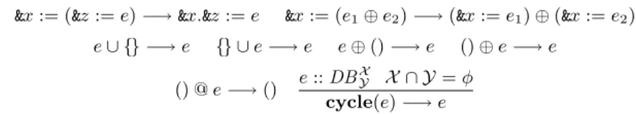
Apart from fusion rules, the following rewriting rules forrecare proposed in [4] for optimizations. Type ofeis assumed to beDBZZ. They simplify the argument ofrecand increases chances of fusions.
rec(λ($l,$t).e)({}) =1⊕
&z∈Z&z :={}
rec(λ($l,$t).e)({l:d}) =e[l/$l][d/$t]@rec(λ($l,$t).e)(d)
rec(λ($l,$t).e)(d1∪d2) =rec(λ($l,$t).e)(d1)∪rec(λ($l,$t).e)(d2) rec(λ($l,$t).e)(&x :=d) =&x :=2(rec(λ($l,$t).e)(d))
rec(λ($l,$t).e)(&x) =⊕
&z∈Z&z :=&y.&z
rec(λ($l,$t).e)() = ()
&x:= (&z:=e)−→&x.&z:=e &x:= (e1⊕e2)−→(&x:=e1)⊕(&x:=e2)
e∪ {} −→e {} ∪e−→e e⊕()−→e ()⊕e−→e
() @e−→() e::DB X
Y X ∩ Y=φ
cycle(e)−→e
Fig. 4.Auxiliary rewriting rules
The first rule eliminatesrec, while the second rule eliminates an edge from the argument.
$t does not occur free ine
rec(λ($l,$t).e)(d1@d2) =rec(λ($l,$t).e)(d1)@rec(λ($l,$t).e)(d2)
$t does not occur free ine
rec(λ($l,$t).e)(cycle(d)) =cycle(rec(λ($l,$t).e)(d))
Additional rules proposed by (full version of) Hidaka et al. [7] to further simplify the body ofrecare given in Fig. 4. The rules in the last line in Fig. 4 can be generalized by static analysis of the marker in the following section. And given the static analysis, we can optimize further as described in Sect. 4.
3
Enhanced Static Analysis
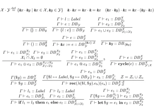
This section proposes our enhanced marker analysis. Figure 5 shows the proposed markerinferencerules for UnCAL. Static environmentΓ denotes mapping from variables to their types. We assume that the types of free variables are given. Since we focus on graph values, we omit rules for labels. Roughly speaking,
DBXY is a type for graphs that haveX input markers exactly and have at most
Y output markers, which will be shown formally by Lemma 1.
The original typing rules were provided based on the subtyping rule
Γ ⊢e::DBXY Y ⊆ Y′
Γ ⊢e::DBXY′
and required the arguments of∪,⊕,if to have identical sets of output markers. Unlike the original rules, the proposed type system does not use the subtyping rule directly for inference. Combined with the forward evaluation semanticsF[[]] that is summarized in [6], we have the following type safety property.
1
Original right hand side was{}in [4], but we corrected here.
2
We overload := in&x :=gto denote renaming of each input marker&z ingto&x.&z.
5
Allowing output marker ofe1ine1@e2that is not included in the input marker ofe2
X · Ydef={&x·&y|&x∈ X,&y∈ Y} &·&x=&x·&=&x (&x·&y)·&z=&x·(&y·&z)
Γ ⊢ {}::DB∅
Γ ⊢l::Label
Γ ⊢e::DBY
Γ ⊢ {l:e}::DBY
Γ ⊢e1::DBXY1 Γ ⊢e2::DBXY2 Γ ⊢e1∪e2::DBXY1∪Y2
Γ ⊢() ::DB∅∅
Γ ⊢e::DBZ Y
Γ ⊢&x :=e::DBY{&x}·Z Γ ⊢&y::DB{&y}
Γ ⊢e1::DBXY11 Γ ⊢e2::DBXY22 X1∩ X2 =∅
Γ ⊢e1⊕e2 ::DBXY11∪X∪Y22
Γ ⊢e1::DBXY11
Γ ⊢e2::DBXY22
Γ ⊢e1@e2::DBXY21
5 Γ ⊢e::DB
X Y
Γ ⊢cycle(e) ::DBXY\X
Γ($g) =DBXY
Γ ⊢$g::DBXY
Γ ⊢ea::DBXY
Γ{$l7→Label,$g7→DBY} ⊢eb::DBZZio Z=Zi∪ Zo
Γ ⊢rec(λ($l,$g).eb)(ea) ::DBX ·ZY·Z
Γ ⊢l1::Label Γ ⊢l2::Label
Γ ⊢et::DBXYt Γ ⊢ef::DB
X Yf Γ ⊢ifl1=l2thenetelseef::DBXYt∪Yf
Γ ⊢e1::DBXY11
Γ{$g7→DBX1
Y1} ⊢e2::DB
X2
Y2 Γ ⊢let$g=e1ine2::DBXY22
Fig. 5.UnCAL Static Typing (Marker Inference) Rules: Rules forLabelare Omitted
Lemma 1 (Type Safety). Assume that g is the graph obtained byg =F[[e]]
for an expression e. Then, ⊢ e :: DBXY implies both inMarker(g) = X and outMarker(g)⊆ Y.
Lemma 1 guarantees that the set of input markers estimated by the type infer-ence is exact in the sense that the set of input markers generated by evaluation exactly coincides with that of the inferred type. For the output markers, the type system provides an over-approximation in the sense that the set of output markers generated by evaluation is a subset of the inferred set of output mark-ers. Since the statement on the input marker is a direct consequence of the rules in [4], we focus that on the output markers and prove it. The proof, which is based on induction on the structure of UnCAL expression, is in Sect. A.2 in the appendix.
4
Enhanced Rewiring Optimization
This section proposes enhanced rewriting optimization rules based on the static analysis shown in the previous section.
4.1 Rule for @ and Revised Fusion Rule
()@e−→() ⇒ e1::DB
X ∅
e1@e2−→e1 (2)
As we have seen in Sect. 2, we have two fusion rules forrec. Although the first rule can be used to gain performance, the second rule is more complex so less performance gain is expected. Using (2), we can relax the condition of the first condition of the fusion rule (1) to increase chances to apply the first rule as follows.
rec(λ($l2,$t2).e2)(rec(λ($l1,$t1).e1)(e0)) =rec(λ($l1,$t1).rec(λ($l2,$t2).e2)(e1))(e0)
ife2 does not depend on $t2, ore1::DBX∅
Here, the underlined part is changed.
4.2 Further Optimization with Static Marker Information
For more general cases of@, we have the following rule.
e1::DBXY1 e2::DB
Y2
Z Y1∩ Y2=∅ RmY1hhe1ii=e
e1@e2−→e
RmYhheiidenotes static removal of the set of output markers. It’s definition will
be given in the next subsection. It is necessary for correctness of the optimization transformation.
4.2.1 Static Output-Marker Removal Algorithm and Soundness
The formal definition ofRmYhheiiis shown below.
Rm∅hheii=e RmX ∪Yhheii=RmYhhRmXhheiiii Rm{&y}hh{}ii={}
Rm{&y}hh()ii= () Rm{&y}hh&yii={} Rm{&y}hh&xii=&x
Rm{&y}hhe1⊙e2ii=Rm{&y}hhe1ii ⊙Rm{&y}hhe2ii (⊙ ∈ {∪,⊕})
Rm{&y}hh&x:=eii= (&x:=Rm{&y}hheii)
Rm{&y}hh{l:e}ii={l:Rm{&y}hheii}
Rm{&y}hhe1@e2ii=e1@Rm{&y}hhe2ii
Rm{&y}hhifbthene1elsee2ii=ifbthenRm{&y}hhe1iielseRm{&y}hhe2ii
Since the output markers of the result of @ are not affected by that of e1, e1 is not visited in the rule of @. In the following, IdYY andBotY∅ is respectively defined as⊕
&z∈Y&z :=&z and
⊕
&z∈Y&z :={}.
e::DBXY &y∈(Y \ X)
Rm{&y}hhcycle(e)ii=cycle(Rm{&y}hheii)
e::DBXY &y ∈/ (Y \ X)
Rm{&y}hhcycle(e)ii=cycle(e)
$v ::DBXY &y ∈ Y/
Rm{&y}hh$vii= $v
$v::DBXY &y ∈ Y
Rm{&y}hh$vii= $v@(Bot{
&y} ∅ ⊕Id
The first rule of $v says that according to the safety of type inference, &y is guaranteed not to result at run-time, so the expression $v remains unchanged. The second rule actually removes the output marker&yj, but static removal is impossible. So the removal is deferred till run-time. The output node marked&yj is connected to node produced by&y :={}. Since the latter node has no output marker, the original output marker disappears from the graph produced by the evaluation. The rest of the &yk :=&yk does no operation on the marker. Since estimationYis the upper bound, the output maker may not be produced at run-time. If it is the case, connection withε-edge by@does not occur, and the nodes produced by the := expressions are left unreachable, so the transformation is still valid. As another side effect, @ may connect identically marked output nodes to single node. However, the graph before and after this “funneling” connection are bisimilar, since every leaf node with identical output markers are bisimilar by definition. Should the output nodes are to be further connected to other input nodes, the target node is always single, because more than one node with identical input marker is disallowed by the data model. So this connection does no harm. Note that the second rule increases the size of the expression, so it may increase the cost of evaluation.
rec(λ($l,$t).eb)(ea) ::DBX ·ZY·Z &y ∈ Y
Rm{&y.&z|&z∈Z}hhrec(λ($l,$t).eb)(ea)ii=rec(λ($l,$t).eb)(Rm{&y}hheaii)
Forrec, one output marker&y ineacorresponds to{&y} · Z={&y.&z |&z ∈ Z}
in the result. So removal of &y from ea results in removal of all of the{&y} · Z. So only removal of all of{&y.&z |&z ∈ Z}at a time is allowed.
Lemma 2 (Soundness of Static Output-Marker Removal Algorithm).
Assume that G = (V, E, I, O) is a graph obtained by G= F[[e]] for an expres-sion e, and e′ is the expression obtained by Rm
Yhheii. Then, we have F[[e′]] =
(V, E, I,{(v,&y)∈O|&y ∈ Y}/ ).
Lemma 2 guarantees that no output marker inY appers at run-time ifRmYhheii
is evaluated.
4.2.2 Plugging Expression to Output Marker Expression
The following rewriting rule is to plug an expression into another through cor-respondingly marked node.
{l:&y}@ (&y:=e)−→ {l:e}
This kind of rewriting was actually implicitly used in the exemplification of optimization in [4], but was not generalized. We can generalize this rewriting as
e@ (&y:=e′)−→
{
RmY\&yhheii[e′/&y] if&y ∈ Y wheree::DBXY
RmYhheii otherwise.
where e[e′/&y] denotes substitution of &y bye′ ine. Since nullrary constructors
no effect and the rule in the latter case apply. So we focus on the former case in the sequel. For most of the constructors the substitution rules are rather straightforward:
&y[e/&y] =e
(e1⊙e2)[e/&y] = (e1[e/&y])⊙(e2[e/&y]) (⊙ ∈ {∪,⊕}) (&x:=e)[e′/&y] = (&x:= (e[e′/&y]))
{l:e}[e′/&y] ={l: (e[e′/&y])}
(e1@e2)[e/&y] =e1@ (e2[e/&y])
(ifbthene1elsee2)[e/&y] =ifbthen(e1[e/&y])else(e2[e/&y])
Since the final output marker for@is not affected by that ofe1,e1is not visited in the rule of@. Forcycle, we should be careful to avoid capturing of marker.
cycle(e)[e′/&y] = {
cycle(e[e′/&y]) if (Y′∩ X) =∅wheree::DBX
Y e′::DBY′
cycle(e)[e′/&y] otherwise.
The above rule says that if &y will be a “free” marker in e, that is, the output markers ine′, namelyY′ will not be captured bycycle, then we can pluge′ into
output marker expression ine. If some of the output markers inY′are included
in X, then the renaming is necessary. As suggested in the full version of [3], markers inX instead of those inY′ should be renamed. And that renaming can
be compensated outside ofcycleas follows:
cycle(e)def= (⊕
&x∈X
&x:=&tmpx) @cycle(e[&tmpx1/&x1]. . .[&tmpxM/&xM])
where &x1, . . . ,&xM = X are the markers to be renamed, and X of e :: DBXY is used. Note that in the renaming, not only output markers, but also input markers are renamed. &tmpx1, . . . ,&tmpxM are corresponding fresh (temporary)
markers. The left hand side of@recovers the original name of the markers. After renaming bycycle, no marker is captured anymore, so substitution is guaranteed to succeed. For variable reference and rec, static substitution is impossible. So we resort to the following generic “fall back” rule.
e∈ {$v,rec( )( )} e::DBXY Y={&y1, . . . ,&yj, . . . ,&yn}
e[e′/&yj] =e@ (
&y1:=&y1, . . . ,&yj−1:=&yj−1,&yj:=e′,
&yj−1:=&yj−1, . . . ,&yn:=&yn
)
The “fall back” rule is used for rec because unlike output marker removal algorithm, we can not just plug e into ea since that will not plug e but rec(λ($l,$t).eb)(e) in the result. We could have used the inverserec(λ($l,$t).eb)−1 to plugrec(λ($l,$t).eb)−1(e′) instead, but the inverse does not always exist in
general.
then apply functionF that implements−→and other rewriting rules recursively such as fusions described in this paper, on the result ofP.
With respect to proposed rewriting rules in this section, the following theorem hold.
Theorem 1 (Soundness of Rewriting). If e −→e′, thenF[[e]] is bisimilar
toF[[e′]].
It can be proved by simple induction on the structure of UnCAL expressions, and omitted here.
Example 4. The following transformation that apply selection afterconsecutive
in Example 3
rec(λ($l1,$g1).if$l1=athen{$l1: $g1}else{})(consecutive($db)) is rewritten as follows:
{expand definition ofconsecutive and apply 2nd fusion rule}
=
rec(λ($l,$g).rec(λ($l1,$g1).if$l1=athen{$l1: $g1}else{}) (rec(λ($l′,$g′).if$l = $l′ then{result: $g′}else{})($g)
@rec(λ($l,$g).rec(λ($l′,$g′).
if$l= $l′then{result: $g′}else{})($g))($g)))($db)
{ (2)}
= rec(λ($l,$g).rec(λ($l1,$g1).if$l1=athen{$l1: $g1}else{}) (rec(λ($l′,$g′).if$l = $l′ then{result: $g′}else{})($g)))($db)
{ 2nd fusion rule, (2),recrule forif and{l:d}, static label comparison}
= rec(λ($l,$g).rec(λ($l′,$g′).{})($g))($db)
This example demonstrates the second fusion rule promotes to the first. The top level edges of the result ofconsecutive are always labeled resultwhile the selection selects subgraphs under edges labeled a. So the result will always be empty, and correspondingly the body ofrecin the final result is{}.
More examples can be found in Sect. A.3 in the appendix.
5
Implementation and Performance Evaluation
This section reports preliminary performance evaluations.
5.1 Implementation in GRoundTram
Table 1.Summary of experiments (running time is in CPU seconds)
direction no rewriting previous [4, 7] ours
Class2RDBforward 1.18 0.68 0.68
backward 14.5 7.99 7.89
PIM2PSM forward 0.08 0.77 (2*3) 0.07 (2*13)
backward 1.62 3.64 0.75
C2Osel forward 0.04 0.04 (2*1) 0.05 (2*11)
backward 2.26 0.26 0.27
C2Osel’ forward 0.05 0.06 (2*1) 0.04 (2*11)
backward 2.53 2.58 1.26
UnQL forward 0.022 0.016 (1*1) 0.010 (1*1)
backward 0.85 0.30 0.15
5.2 Performance Results
Performance evaluation was conducted on GRoundTram, running on MacOSX over MacBookPro 17 inch, with 3.06 GHz Intel Core 2 Duo CPU. Time com-plexity is PTIME for the size of input graph[4], and exponential in the size (number of compositions or nesting of recs) of the transformation. In the ex-periments, the size of input data (graph) is not very large (up to a hundred of nodes).
Table 1 shows the experimental results. Each running time includes time for forward and backward transformations [6], and for backward transforma-tions, algorithm for edge-renaming is used, and no modification on the target is actually given. However, we suppose presence of modification would not make much difference in the running time. Running time of forward transformation in which rewriting is applied (last two columns) includes time for rewriting. Rewrit-ing took 0.006 CPU seconds at the worst case (PIM2PSM, ours). Class2RDB
stands for class diagram to table diagram transformation, PIM2PSMfor plat-form independent model to platplat-form specific model transplat-formation, C2Osel is for transformation of customer oriented database into order oriented database, followed by a simple selection, andUnQLis the example that is extracted from our previous paper [7], which was borrowed from [4]. It is a composition of two recs. Concrete plugging optimizations in this example can be traced in Sect. A.3 in the appendix.
The numbers in parentheses show how often the fusion transformation hap-pened. For example,PIM2PSM led to 3 fusions based on the second rule, and further enhanced rewriting led to 10 more fusion rule applications, all of which promoted to the first rule via proposed rewriting rule (2). Same promotions happened toC2Osel. Except forC2Osel’, a rtime optimization in which un-reachable parts are removed after every application ofrecis applied. Enhanced rewriting led to performance improvements in both forward and backward eval-uations, exceptC2Osel. Comparing “previous” with “no rewriting”, PIM2PSM
fusion turns composition of recs to their nesting. In the presence of the run-time optimization, composition is advantageous than nesting when only small part of the result is passed to the subsequent recs, which will run faster than when passed entire results (including unreachable parts). Once nested, interme-diate result is not produced, but the run-time optimization is suppressed because every execution of the inner rec traverses the input graph.C2Osel’in which run-time optimization is turned off, shows that the enhanced rewriting itself lead to performance improvements.
6
Related Work
Some optimization rules were mentioned in [7], but relationship with static marker analysis was not covered in depth. By enhanced marker analysis and rewriting rules in present paper, all the rules in [7] can be generalized uniformly. An implementation of rewriting optimizations was reported in [6] but con-crete strategies were not included in the paper.
Full (technical report) version of [3] dealt with plugging constructor-only expressions into output marker expressions. It was motivated by authors need to express semantics of@at the constructor expression level and not graph data level as in [4]. It also mentioned renaming of markers to avoid capture of the output markers in the cycle expressions6. We do attempt the same thing at the expression level but we argue here more formally.
The technical report also mentioned the semantics ofrec on the cycle con-structor expressions, even when the body expressions refer to graph variables, although marker environment that maps markers to connected subgraphs in-troduced there makes the semantics complex. The journal version [4] did not include this semantics on the cycle constructor expressions. But we could use the semantics to enhance rewriting rules forrecwithcyclearguments.
The journal version mentioned run-time evaluation strategy in which only necessary components of strucural recursion is executed. For example, only&z1 component of recin &z1@rec( )( ) is evaluated.
A static analysis of UnCAL was described in [1], but the main motivation was to analyze structure of graphs using graph schema.
7
Conclusion
In this paper, under the context of graph transformation using UnCAL graph algebra, enhanced static marker inference is first formalized. Fusion rule becomes more powerful thanks to the static marker analysis. Further rewriting rules based on this inference are also explored. Marker renaming for capture avoidance is formalized to support the rewriting rules.
6
In the technical report, cycle was represented by parallel equations, without cycle
Preliminary performance evaluation shows the usefulness of the optimiza-tion for various non-trivial transformaoptimiza-tions in the field of software engineering research.
Under the context of bidirectional graph transformations [6], one of the ad-vantage of static analysis is that we can keep implementation of bidirectional in-terpreter intact. Future work under this context includes reasoning about effects on the backward updatability. Although rewriting preserves well-behavedness of bidirectional transformations, backward transformation before and after rewrit-ing may accept different update operations. Our conjecture is that simplified transformation accepts more updates, but this argument requires further discus-sions.
Acknowledgments We thank reviewers and Dr. Kazuyuki Asada for their
thor-ough comments on earlier versions of the paper. The research was supported in part by the Grand-Challenging Project on “Linguistic Foundation for Bidirec-tional Model Transformation” from the NaBidirec-tional Institute of Informatics, En-couragement of Young Scientists (B) of the Grant-in-Aid for Scientific Research No. 20700035.
References
1. A. A. Bencz´ur and B. K´osa. Static analysis of structural recursion in semistructured databases and its consequences. InADBIS, pages 189–203, 2004.
2. P. Buneman, S. Davidson, M. Fernandez, and D. Suciu. Adding structure to un-structured data. InICDT, volume 1186 ofLNCS, pages 336–350, 1997.
3. P. Buneman, S. Davidson, G. Hillebrand, and D. Suciu. A query language and optimization techniques for unstructured data. InSIGMOD, pages 505–516, 1996. 4. P. Buneman, M. F. Fernandez, and D. Suciu. UnQL: a query language and algebra for semistructured data based on structural recursion.VLDB J., 9(1):76–110, 2000. 5. K. Ehrig, E. Guerra, J. de Lara, L. Lengyel, T. Levendovszky, U. Prange, G. Taentzer, D. Varr´o, and S. Varr´o-Gyapay. Model transformation by graph transformation: A comparative study. Presented at MTiP 2005. http://www.inf.mit.bme.hu/FTSRG/Publications/varro/2005/mtip05.pdf, 2005. 6. S. Hidaka, Z. Hu, K. Inaba, H. Kato, K. Matsuda, and K. Nakano.
Bidirection-alizing graph transformations. In ACM SIGPLAN International Conference on Functional Programming, pages 205–216. ACM, 2010.
7. S. Hidaka, Z. Hu, H. Kato, and K. Nakano. Towards a compositional approach to model transformation for software development. InSAC 2009, pages 468–475, 2009.
8. G. Rozenberg, editor. Handbook of Graph Grammars and Computing by Graph Transformations, Volume 1: Foundations. World Scientific, 1997.
9. I. Sasano, Z. Hu, S. Hidaka, K. Inaba, H. Kato, and K. Nakano. Toward bidirec-tionalization of ATL with GRoundTram. InICMT, June 2011. To appear. 10. P. Stevens. Bidirectional model transformations in QVT: Semantic issues and open
questions. InMoDELS 2007, pages 1–15, 2007.
11. P. Wadler. Deforestation: Transforming programs to eliminate trees. In
A
Appendix
A.1 UnCAL Original Static Typing Rules
a∈ U
a:Label
ya label variable
y:Label
ta tree variable of typeTreeX
t:TreeX
{}:TreeX
X∈ X
X:TreeX
l:Label Q:TreeX
{l⇒Q}:TreeX
l1:Label l2:Label
l1=l2:Bool
l1:Label . . . ln:Label pa variable
p(l1, . . . , ln) :Bool
b:Bool Q1:TreeX Q2:TreeX
ifbthenQ1elseQ2:TreeX
Q1 :TreeY . . . Qm:TreeY
(X1:=Q1, . . . , Xm:=Qm) :Tree{
X1,...,Xm}
Y
Q1:TreeX Q2 :TreeX
Q1∪Q2:TreeX
Q1:TreeX Q2:TreeXY
Q1@XQ2:TreeY
ylabel variable ttree variable of typeTreeY Q1:TreeXX Q2:TreeY gextX(λ(y, t).Q1)(Q2) :TreeXX ·Y
Fig. 6.UnCAL Original Static Typing Rules (TR ver. of [2])
Note thatgextis an old notation of structural recursionrec.
A.2 Proof of Lemma 1 (Refined Type Sefety)
The proof of Lemma 1 is based on induction on the structure of UnCAL expres-sion.
Proof. Base case:
Free variables: We assume that the type of free variables such as $db (input
of the entire transformation) is available.
{}: By the definition of F[[{}]], outMarker(g) = ∅. By the type inference rule,
{}::DB∅. Therefore,∅=outMarker(g)⊆ Y=∅.
&y : outMarker(F[[&y]]) = {&y} and &y :: DB{{&y}. &y :: DB{&y}. Therefore,
{&y} =outMarker(g)⊆ Y ={&y}. Another nullrary constructor(): is treated similarly.
Inductive case:
{l:e}: Supposee::DBY,F[[e]] =g, andF[[{l:e}]] =g′. ThenoutMarker(g′) =
outMarker(g) by the definition ofF[[]] and {l:e}:: DBY by the type inference rule. Now suppose outMarker(g)⊆ Y as an induction hypothesis. Then we have
outMarker(g) =outMarker(g′)⊆ Y.&m :=eis treated similarly.
F[[e1 ∪e2]] = g′. Then outMarker(g′) = outMarker(g1) ∪ outMarker(g2) by
the definition of F[[]] and e1∪e2 :: DBY1∪Y2 by the type inference rule.
Now suppose outMarker(g1) ⊆ Y1 and outMarker(g2) ⊆ Y2 as induction hy-potheses. Then, by the property of the set union, we have outMarker(g′) =
outMarker(g1)∪outMarker(g2) ⊆ Y1∪ Y2. ⊕ is treated similarly because type inference and evaluation rules for the output markers are identical to those of
∪.
e1@e2: Suppose e1 :: DBXY1, e2 :: DBZY2, F[[e1]] = g1, F[[e2]] = g2, and
F[[e1@e2]] = g′. Then outMarker(g′) = outMarker(g2) by the definition of F[[]]
and e1@e2 :: DBXY2 by the type inference rule. Observe that (after
connect-ing with matchconnect-ing input markers in g2) the output markers in g1 are ignored. Now suppose outMarker(g2) ⊆ Y2 as an induction hypothesis. Then we have
outMarker(g′) =outMarker(g2)⊆ Y2.
cycle(e): Supposee::DBXY,F[[e]] =g, andF[[cycle(e)]] =g′. ThenoutMarker(g′) =
outMarker(g)\inMarker(g) by the definition ofF[[]] andcycle(e) ::DBY\Xby the
type inference rule. Now supposeoutMarker(g)⊆ Y as an induction hypothesis. Then, since X = inMarker(g) by the exactness of input marker inference, we have outMarker(g′) =outMarker(g)\inMarker(g)⊆ Y \ X.
ifbthene1elsee2: Suppose e1::DBXY1,e2 ::DB
X
Y2,F[[e1]] =g1,F[[e2]] =g2,
and F[[ifb then e1 else e2]] = g′. Then, depending on the value of b,
outMarker(g′) = outMarker(g1) or outMarker(g′) = outMarker(g2) by the
def-inition of F[[]] and ifbthene1elsee2 :: DBXY1∪Y2 by the type inference rule.
Now supposeoutMarker(g1)⊆ Y1andoutMarker(g2)⊆ Y2as induction hypothe-ses and do case analysis for b. Ifb =true, thenoutMarker(g′) =outMarker(g1),
so outMarker(g′) = outMarker(g1) ⊆ Y
1. For the other case, outMarker(g′) =
outMarker(g2)⊆ Y2. For either case, by the property of the set union, we have
outMarker(g′)⊆ Y1∪ Y2.
rec(λ($l,$t).eb)(ea) : Suppose ea :: DBXY, F[[ea]] = g, eb :: DBZZi
o, and F[[rec(λ($l,$t).eb)(ea)]] =g′. Then,outMarker(g′) ={&y.&z |&y ∈outMarker(g),&z ∈ Z} by the definition of F[[]] where Z = Zi ∪ Zo, and rec(λ($l,$t).eb)(ea) ::
DBX ·ZY·Z by the type inference rule. Now supposeoutMarker(g)⊆ Y as induction hypotheses. Then we have outMarker(g′) = {&y.&z | &y ∈ outMarker(g),&z ∈
Z} ⊆ {&y.&z |&y ∈ Y,&z ∈ Z}. Observe that F[[]] does not use set of markers produced by eb at run-time. Readers may wonder how the output markers are accessed via graph variable t, i.e., Y bound by rec affect the final result. Buneman et al. [4] does not explicitly mention, but it is natural to interpret as follows: UsuallyY is disjoint fromZiand therefore the output nodes marked by
Y are not connected to S1 node7. Therefore we can safely ignore suchY ineb. Bound Variables: Variable $t is introduced byrec(λ($l,$t).eb)(ea) and $t is bound to each of the subgraphs reachable from each edge. Similarly to [4], the type inference rule estimates the output markers as identical to that forea. So assuming type safety forea, type safety for $t immediately follows.
The above analysis covers all the expressions and thus conclude the proof. ⊓⊔
7
A.3 Concrete Rewriting Examples
This section shows input and ouput of optimizations used in “UnQL” trans-formation appeared in Sect. 5. For input transtrans-formation Q1, our system pro-ducesQ2by applying first fusion rule. Previously the translation fromQ2toQ3 was not automatic, but algorithm in Sect. 4 enables derivingQ3automatically.
Q3can be obtained by the plugging based rewriting rules. For example,
(&z1 := (&z1 := {"name": &z2}, &z2 := {"name": &z2})) @ (&z2 := &z1&z2, &z1 := &z1&z1)
becomes
&z1 := (&z1 := {"name": &z1&z2}, &z2 := {"name": &z1&z2}).
This pattern frequently appears after rec fusion because recoften appears in the pattern &z @rec( )( ) because from the UnQL surface syntax, only one component of structural recursion is necessary and the idiom&z@ implements this projection.
Q 1.
&z1@rec(\ ($L,$T). if $L = "name"
then (&z1 := {"name": &z2}, &z2 := {"name": &z2})
else (&z1 := &z1, &z2 := {$L: &z2})) (&z1@rec(\ ($L,$T).
if $L = "name"
then (&z1 := {"name": &z1}, &z2 := {"typeName": &z2}) else if $L = "primitiveDataType"
then (&z1 := {"primitiveDataType": &z2}, &z2 := {"primitiveDataType": &z2}) else (&z1 := {$L: &z1}, &z2 := {$L: &z2})) ($db))
Q 2.
&z1@(&z2 := &z1&z2, &z1 := &z1&z1)@ rec(\ (Sa1,$T).
if Sa1="name"
then (&z1 := (&z1 := {"name": &z2}, &z2 := {"name": &z2}) @ (&z2 := &z1&z2, &z1 := &z1&z1),
&z2 := (&z1 := &z1,
&z2 := {"typeName": &z2}) @ (&z2 := &z2&z2, &z1 := &z2&z1)) else if Sa1 = "primitiveDataType"
&z2 := {"primitiveDataType": &z2}) @ (&z2 := &z2&z2, &z1 := &z2&z1),
&z2 := (&z1 := &z1,
&z2 := {"primitiveDataType": &z2}) @ (&z2 := &z2&z2, &z1 := &z2&z1))
else (&z1 := if $Sa1 = "name" then (&z1 := {"name": &z2},
&z2 := {"name": &z2})
else (&z1 := &z1, &z2 := {$Sa1: &z2}) @ (&z2 := &z1&z2, &z1 := &z1&z1),
&z2 := if $Sa1 = "name" then (&z1 := {"name": &z2},
&z2 := {"name": &z2})
else (&z1 := &z1, &z2 := {$Sa1: &z2}) @ (&z2 := &z2&z2, &z1 := &z2&z1)))($db)
Q 3.
&z1@(&z2 := &z1&z2, &z1 := &z1&z1)@ rec(\ ($Sa1,$T).
if $Sa1="name"
then (&z1&z1 := {"name": &z1&z2}, &z1&z2 := {"name": &z1&z2}, &z2&z1 := &z2&z1,
&z2&z2 := {"typeName": &z2&z2}) else if $Sa1 = "primitiveDataType"
then (&z1&z1 := &z2&z1,
&z1&z2 := {"primitiveDataType": &z2&z2}, &z2&z1 := &z2&z1,
&z2&z2 := {"primitiveDataType": &z2&z2} else (&z1 := if $Sa1 = "name"
then (&z1 := {"name": &z1&z2}, &z2 := {"name": &z1&z2}) else (&z1 := &z1&z1,
&z2 := {$Sa1: &z1&z2}), &z2 := if $Sa1 = "name"
then (&z1 := {"name": &z2&z2}, &z2 := {"name": &z2&z2}) else (&z1 := &z2&z1,
![Table 1. Summary of experiments (running time is in CPU seconds) direction no rewriting previous [4, 7] ours](https://thumb-ap.123doks.com/thumbv2/123deta/8631308.449574/16.918.266.652.201.390/table-summary-experiments-running-seconds-direction-rewriting-previous.webp)
![Fig. 6. UnCAL Original Static Typing Rules (TR ver. of [2])](https://thumb-ap.123doks.com/thumbv2/123deta/8631308.449574/19.918.272.672.277.547/fig-uncal-original-static-typing-rules-tr-ver.webp)
